Given two worker processes which start and complete tasks at a service rate of \(\alpha^1\) and \(\alpha^2\) tasks every \(100~\mathrm{ms}\), what is the optimal assignment of tasks to workers that ensures the fastest task completion? Such a choice depends on the current number of tasks each worker is assigned as well as their respective service rates. Consider the following example. Worker 1 performs tasks at rate \(\alpha^1 = 2\) while Worker 2 performs tasks at rate \(\alpha^2 = 1\). Suppose we had to assign a new task to one of these workers. We observe that there are three tasks assigned to Worker 1 and two tasks assigned to Worker 2. The correct choice in this case is to assign the new task to Worker 1 — the fastest worker — since it will only take \(200~\mathrm{ms}\) to complete all the tasks. It is not always best to assign more work to the fastest worker, however. Suppose instead that Worker 1 had four tasks assigned to it. In this case, it is better to assign the new task to Worker 2 because we can finish all the tasks in \(200~\mathrm{ms}\). Had we assigned the task to Worker 1, it would take \(300~\mathrm{ms}\) to complete all the tasks and Worker 2 would be idling in the last \(100~\mathrm{ms}\) period. Is there a formal way to compute this best choice given the current configuration of the system?

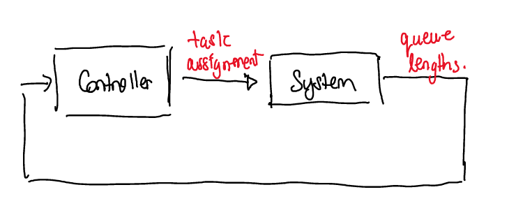
This is a problem of task assignment — assigning tasks to workers to ensure the fastest throughput where a task is assigned exactly once — and it can cast as a problem of control theory. Control theory is the formal study of driving the configuration of a real-world system to a desired configuration by leveraging current information. This is depicted in the diagram below for this problem.

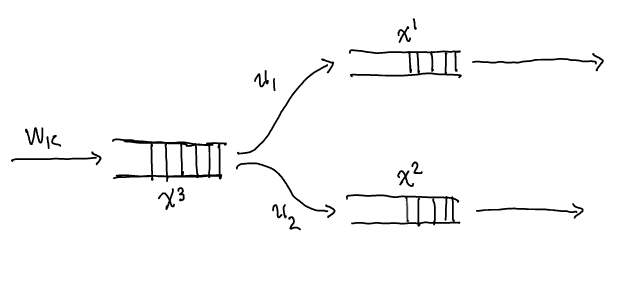
At the start of every \(100~\mathrm{ms}\) period, the control algorithm observes the current state of the queues behind every worker and assigns all unassigned tasks. Then, during the \(100~\mathrm{ms}\) period, every worker completes as many tasks as it can: the minimum of the number of tasks in its queue and its service rate. We can describe this mathematically. Formally, let \(x^1_k\), \(x^2_k \in \mathbb{Z}_{\geq 0}\) be the number of tasks assigned to Worker 1 and 2 respectively at period \(k\) and let \(x^3_k \in \mathbb{Z}_{\geq 0}\) be the number of unassigned tasks at the start of period \(k\). Let \(u^1_k\), \(u^2_k \in \mathbb{Z}_{\geq 0}\) denote the number of additional tasks to assign to Worker 1 and 2 respectively at the start of period \(k\). Define \[ f(x_k, u_k, w_k) = \left( \begin{array}{l} \max\{0, x^1_{k} - \alpha^1 + u^1_k\}\\ \max\{0, x^2_{k} - \alpha^2 + u^2_k\}\\ \max\{0, x^3_{k} - u^1_k - u^2_k + w_k\} \end{array} \right). \] The number of tasks changes from period \(k\) to period \(k+1\) according to the following discrete-time law, \[ x_{k+1} = f(x_k, u_k, w_k), \] where \(w_k\) denotes the (unknown) number of new unassigned tasks. For now assume \(w_k = 0\): suppose we need only service \(x^3_0\) tasks for all time (a finite number). The \(\max\) ensures that we do not service more tasks than are actually queued behind a worker. The diagram below depicts the mathematical law.

Let \(y^i_k\) denote the number of tasked serviced by worker \(i\) at time period \(k\). It is given by the expression \[ y^i_k = \min\{x^i_k + u^i_k, \alpha^i\}. \] If this quantity is less than \(\alpha^i\), then worker \(i\) is under-utilized. The number of steps required to clear both worker queues is, \[ \max\left\{\frac{x^1_{k}}{\alpha^1}, \frac{x^2_{k}}{\alpha^2} \right\}. \] Together we use these quantities to solve for the policy that ensures the queues are cleared as quickly as possible. Consider the optimization problem, \[ \begin{array}{cl} \max & \sum_{i=0}^{\infty} y^i_k - \max\left\{\frac{x^1_{k}}{\alpha^1}, \frac{x^2_{k}}{\alpha^2} \right\}\\ \text{s.t.} & 0 = x_{k+1} - f(x_k, u_k, w_k)\\ & 0 = w_k\\ & 0 = x_0 - (s^1_0, s^2_0, s^3_0) \end{array} \] that maximizes a reward function with the aim of finding a task assignment that achieves:

• the largest number of tasks are serviced at any given time, and
• the shortest amount of time is spent servicing all the tasks,

given a known initial state \((s^1_0, s^2_0, s^3_0)\).

The aforementioned goals work together. Increasing the number of serviced tasks in a given moment cannot increase the amount of time taken to clear all other tasks. Likewise, decreasing the number of steps taken to clear the queues cannot decrease the amount of tasks serviced at any given time. It stands to reason that a task assignment that solves this optimization problem solves our task assignment problem. Note, such a solution depends on the initial condition \((x^1_0, x^2_0, x^3_0)\) which importantly includes the number of tasks waiting on each worker.

Note: The \(y^i_k\) terms seem superfluous, but are in fact critical in ensuring the optimization produces the correct solution. Without the \(y^i_k\) terms, the trivial task assignment (i.e. \(u = 0\)) maximizes the reward. These terms ensure that tasks are actually serviced.

The optimization could be solved by iterating over all possible choices for \(u_k\), but this would be very expensive. To avoid this, we recast this problem as a problem of graph theory. We consider the graph where each node in the graph is a configuration of the system (number of tasks in all the queues) at a given time. Each edge corresponds to a task assignment at that given time and how transfers the current configuration to the next configuration. Such a graph has a structure that looks like,

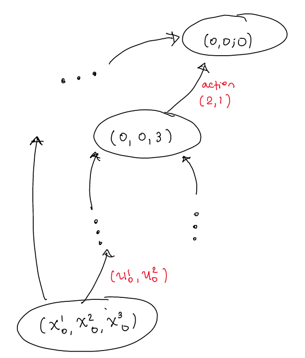
The cost of each edge is precisely the contribution \[ y^1_k + y^2_k - \max\left\{\frac{x^1_{k+1}}{\alpha^1}, \frac{x^2_{k+1}}{\alpha^2}\right\}, \] which is added by that transition to the overall reward in the complete optimization problem. The problem of finding the highest reward path from an initial configuration (the current one) to \((0, 0, 0)\) is precisely the problem we aim to solve. Dijkstra’s Algorithm can be used to find the optimal path.

Note: Dijkstra’s Algorithm relies on having a finite number of out-edges from any given node. This is assured in this problem by the fact that \(u^i_k\) has a lower and upper bound. The relationship between \(x^3_{k+1}\) and \(x^3_{k}\) enforce this bound. This is normally the case in In software applications. A different approach (usually analytic) is used in the control of physical systems where the control action lay in a continuum (\(\mathbb{R}\)).

To evaluate the performance of this method, we can simulate the mathematical system \((1)\) with different policies. We will call the policy constructed above the ``reward-based’’ policy. I compare this reward-based policy against two other policies:

• Round Robin: Cycle between workers for each task.
• Weighted Scheme: Choose which worker gets a task based on how much work was assigned in the past. If Worker 1 works twice as fast as Worker 2, then Worker 1 is assigned twice as many tasks as Worker 2 on average.

The weighted scheme replicates the implementation of Apache’s By Request load balancing module in Apache’s HTTP server httpd. It is an open-loop policy: it does not rely on the current state of the worker queues. In essence, it keeps a tally of which workers are overassigned or underassigned tasks relative to a weight. This tally is used to assign tasks to underassigned workers.

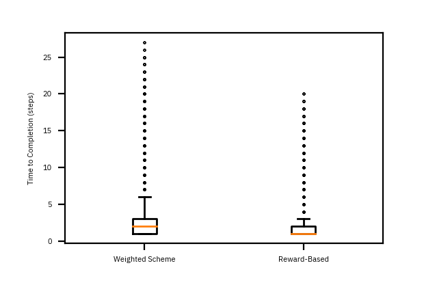
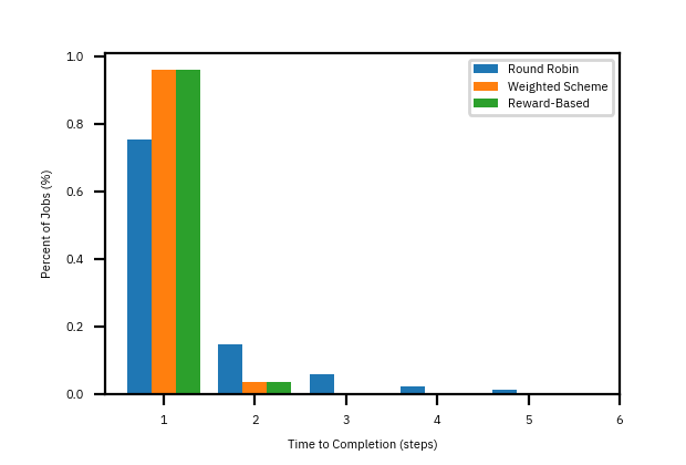
Unlike in the design above, the simulation samples the number of tasks \(w_k\) that need to be assigned from a Poisson distribution. The average arrival rate of tasks is \(6\) per period. In this simulation, the average arrival rate is \(6\) per step with service rates \(\alpha_1 = 6\) and \(\alpha_2 = 3.\) Figure 1 depicts the distribution of task completion times. The reward-based policy is indistinguishable from the performance of open-loop weighted scheme. On the other hand, round-robin policy fairs quite poorly.

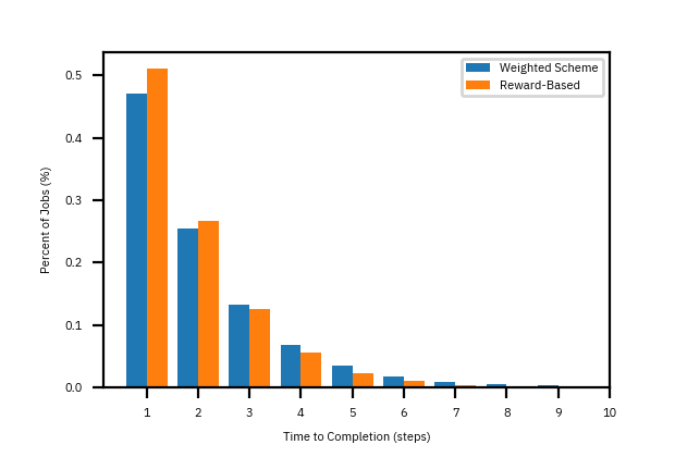
The real advantage in using feedback is when there is uncertainty in the service rates — there is noise in the loop! Suppose the service rates \(\alpha_1\) and \(\alpha_2\) varied with a known average rate for each worker. This could be because the actual amount of time to complete a task varies. As Figure 2 demonstrates, the reward-based policy improves the performance of at least 5% of tasks. However, there is a more visible effect in the nature of outliers. Figure 3 shows that the extent of the distribution and its outliers. Notice that the spread of distribution is greatly reduced with the reward-based policy.