Formally Designing a Gacha System
We want to design a system that allows a video game player to spend in-game currency in exchange for a chance at acquiring rare in-game items, and some default items otherwise. This chance is called a roll. Rare items should, of course, come about less often through this randomized system, but we also do not want to torture players by making it nearly impossible to acquire these rare items. This specification will become important later. As a start, we impose a guarantee on when a “win” will happen by.
Problem Specification
Here is an example specification. Define three categories of items: Default, Rare, and Ultra-Rare. We would like to meet the following specifications:
- Players will receive a rare (or higher) item within \(10\) rolls.
- Players will receive an ultra-rare item within \(90\) rolls.
- For a sufficiently large number of rolls: Of the total amount of rolls, \(1.6\%\) of them will be ultra-rare items.
- For a sufficiently large number of rolls: Of the total amount of rolls, \(13\%\) of them will be rare items.
An excellent framework for setting up this design is a Markov Chain. A Markov Chain is a model that pairs a state with a transition probability where the probability of moving from one state to another is determined solely on the current state.
There is a natural choice of state for this problem. Define the state as the tuple \((x_r, x_u)\) where \(x_r\) is the number of rolls acquiring a rare (or higher) item, and \(x_u\) is the number of rolls since acquiring an ultra-rare item. So, for example, we are in state \((0, 1)\) if we acquired a rare item in the last roll, and an ultra-rare item on the roll prior to that. Because of specification (1) we have \(x_r\) \(\in\) \(\{0,\) \(\ldots,\) \(9\}\) and, because of specification (2), \(x_u\) \(\in\) \(\{0,\) \(\ldots,\) \(89\}.\) The number of total states is then just product of these individual state-spaces: a total of \(900\) states. Not all of these states are connected since the player will perform one roll at a time. For example, you can only jump from \((3, 4)\) to one of: \((0, 0)\) (won an ultra-rare item), \((0, 5)\) (won a rare item) and \((4, 5)\) (won the default item). So, although the state-space is massive, the number of transitions is actually quite small and is only \(3\) times the number of states: we only need to characterize these probabilities.
To keep things simple, we start by setting the probability of acquiring an ultra rare item to be the exact same on every roll on the \(90\)th roll — this last roll has probability \(1\) of acquiring an ultra-rare item. Call the base probability \(\alpha_u \in (0, 1).\) Similarly, we set the probability of acquiring a rare item to be the exact same on every roll on the \(10\)th pull — this last roll has probability \(1\) of acquiring a rare ultra-rare item. Note this doesn’t fully specify the transition probability. Call the base probability \(\alpha_r \in (0, 1)\) for acquiring a rare item.
We are now ready to take care of the easy transition cases. Suppose \(x_r < 9\) and \(x_u < 89.\) In these cases, we do not need to worry about specification (1) and (2) as we haven’t reached the states where we provide a guaranteed win. We have the following transition probabilities,
| Transition | Probability | Meaning |
|---|---|---|
| \((x_r, x_u) \to (0, 0)\) | \(\alpha_u\) | Won an Ultra-Rare Item |
| \((x_r, x_u) \to (0, x_u + 1)\) | \(\alpha_r\) | Won a Rare Item |
| \((x_r, x_u) \to (x_r + 1, x_u + 1)\) | \(1 - \alpha_u - \alpha_r\) | Won a Default Item |
If the player wins an ultra-rare item, then the state must transition to \((0, 0)\) which describes that there have been \(0\) rolls since a rare or higher item was won. If the player wins a rare item, then the state transitions to \((0, x_u + 1)\) since there will be \(0\) rolls since a rare item was won, but \(x_u + 1\) since an ultra-rare item was won. The last case is the default, where the player wins the default item and both the number of rolls since winning a rare and ultra-rate item increase.
Now for the edge cases. If \(x_u = 89,\) then there is a probability \(1\) transition to \((0, 0),\) because of specification (2) and there is no other transition from this state. If \(x_r = 9\) and \(x_u < 89,\) then there is a probability \(1\) chance of acquiring a rare or ultra rare item. Technically, specification (1) is incomplete since it does not indicate what the relative probability between the rare or ultra-rate item is. To keep things simple again, we keep those probabilities in ratio. That is,
| Transition | Probability | Meaning |
|---|---|---|
| \((9, x_u) \to (0, 0)\) | \(\frac{\alpha_u}{\alpha_u + \alpha_r}\) | Won an Ultra-Rare Item |
| \((9, x_u) \to (0, x_u + 1)\) | \(\frac{\alpha_r}{\alpha_u + \alpha_r}\) | Won a Rare Item |
This fully specifies the structure of our Markov chain, but we still do not know the tuning parameters \(\alpha_r\) and \(\alpha_u.\)
Specifications (3) and (4) impose constraints that determine these parameters. How? It is possible, given the transition probabilities above for a Markov chain, to compute the proportion of states where we reside in any given state. This is known formally as the stationary distribution of the Markov chain. It is not necessarily unique, but it is in this particular problem setup — the graph associated to our Markov chain is strongly connected. The stationary distribution can be computed numerically. If we write the above probabilities in what is known as a probability transition matrix \(P \in \mathbb{R}^{900\times 900},\) then the left eigenvector of \(P\) associated to the eigenvalue \(1\) provides this information. Element \(i\) of this eigenvector indicates the ratio between transitions to state \(i\) versus the total number of state transitions.
Specification (3) essentially demands that the ratio of transitioning into \((0, 0)\) — winning an ultra-rare item — to the total number of transitions — total rolls — is \(1.6\%.\) Specification (4) demands that the ratio of transitioning into the states of the form \((0, x_u)\) with \(x_u > 0\) — winning a rare or higher item that is not ultra-rare — to the total number of transitions is \(13\%.\) One can cast finding \(\alpha_u\) and \(\alpha_r\) as an optimization problem that minimizes the distance between the left eigenvector meeting these objectives. Solving this optimization results in the parameters \[ \alpha_r = 7.63\%, \quad \alpha_u = 0.52\%, \] with a ratio of \(1.6\%\) ultra-rare wins and \(13.01\%\) rare item wins.
Discussion of Probabilities
We are done now, right? Not in my opinion. It is healthy to check the final stationary distribution. The stationary distribution tells us the ratio between transitions to a given state versus the total number of state transitions. Given the very linear structure of our rolling system, we can even use the stationary distribution to infer how many of our wins actually come from any given state. In other words, we can estimate how much time a player must wait before winning. Ideally, they should not spend most of their time waiting til the \(90\)th roll to win an ultra-rare item. Here is the stationary distribution, and the associated cumulative distribution function.
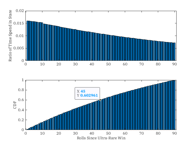
The probability of transitioning into a state between \(45\) and \(89\) rolls since an ultra-rare win is around \(40\%.\) At the tail end, the probability of transitioning into a state between \(70\) and \(89\) rolls since an ultra-rare win is around \(20\%.\) This sounds reasonable doesn’t it? Not really.
In reality, based on the stationary distribution, \(50\%\) of our wins come from the last guaranteed win. This follows from the following reasoning. We spend \(0.008\%\) of our time in state \(89\) and around \(0.015\%\) of our time in state \(10\). We know we must progress from state \(10\) to \(11\) up until \(89\) to reach state \(89\). As a result, about half the time that we are at state \(10\) we know we will make it to state \(89\)! That isn’t great at all.
A Redesign?
Unfortunately, there is no “clean” resolution for this problem. The problem is that the desired ratio of \(1.6\%\) ultra-rare wins is far too close to one over the maximum rolls before a guaranteed win (\(1/90 \approx 1.1\%\)). Even if the state machine provided a win only at the end (\(\alpha_u = 0\)), the rate of ultra-rare wins over rolls will still be \(1.1\%.\) That does not leave much room for early wins without increasing the probability beyond the target \(1.6\%.\)
One “fix” is to simply make it nearly impossible to win before roll \(50,\) and redistribute the likelihood of winning an ultra-rare item between only rolls \(50\) and up. This can be done with a power-law like distribution: instead of \(\alpha_u\) probability at roll \(i,\) the probability will be \(\alpha_u^{90 - i}.\) This does work and will result in practically no wins in the first \(50\) rolls and then a sudden burst of wins around the \(60\) to \(80\) range with almost nobody making it to roll \(90.\)