Solving a system of \(\ell\) partial differential equations (PDE) on \(\mathbb{R}^n\) asks us to find solution functions \(h: \mathbb{R}^n \to \mathbb{R}\) that simultaneously solves the equations \[\begin{aligned} 0 &= \sum_{i = 1}^{n} A_{1, i}(p) \left.\frac{\partial h}{\partial x^i}\right|_{x = p},\\ &\phantom{=} \vdots \\ 0 &= \sum_{i = 1}^{n} A_{\ell, i}(p) \left.\frac{\partial h}{\partial x^i}\right|_{x = p}. \end{aligned}\] The family of functions that solve a system of PDEs can be quite large. It is further restricted by imposing a boundary condition. A boundary condition asks that, on some surface \(\mathsf{N} \subseteq \mathbb{R}^n,\) the solution \(h\) agrees with some known function \(g: \mathsf{N} \to \mathbb{R}.\) That is, \[\left.h\right|_{\mathsf{N}} = g\]

The functions \(A_{j, i}: \mathbb{R}^n \to \mathbb{R}\) and \(g\) are often taken to be real analytic — have a convergent real-valued Taylor series — as this ensures existence and uniqueness of solutions. We will not make this assumption and instead assume these functions have infinitely many continuous derivatives. Such functions are known as simply smooth.

First, let us see how uniqueness fails in this case. Consider the linear partial differential equation on \(\mathbb{R}^3,\) \[0 = \frac{\partial h}{\partial x} - y \frac{\partial h}{\partial z},\] with the boundary condition \[\left. h \right|_{y = 0} = z^3 \lambda(z), \quad \lambda(z) := \left\{ \begin{array}{ll} \exp\left( 1 - \frac{1}{1 - z^2} \right), & z\in(-1, 1)\\ 0. & \text{else} \end{array} \right.\] This is not real-analytic. The smooth functions, \[h_1(x, y, z) = (z + x\, y)^3\,\lambda(z + x\, y),\] \[h_2(x, y, z) = h_1(x, y, z)\, \lambda(2 y) + y,\] and \[h_3(x, y, z) = (y + 1)\, h_2(x, y, z) + 3\,(1 - \lambda(2 y)),\] are smooth solutions that satisfy the boundary condition but clearly disagree on the rest of \(\mathbb{R}^3.\)

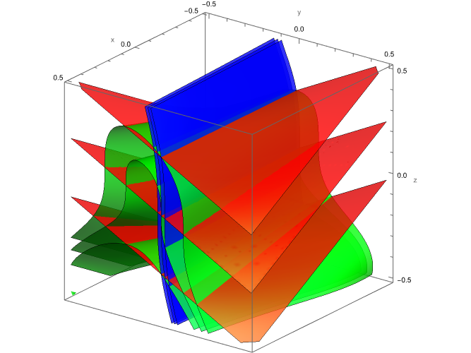
As seen on the boundary in Figure 1, they are even locally, pairwise differentially independent. This should be placed in contrast with linear ordinary differential equations which have global existence and uniqueness of solutions. Even smooth, nonlinear ordinary differential equations have local existence and uniqueness. If we restrict to the real-analytic category of functions, and impose the analytic boundary condition \[\left. h \right|_{y = 0} = z^3,\] then the solution \[h(x, y, z) = (z + x\, y)^3,\] is uniquely determined.

The study of partial differential equations primarily makes this assumption. Partial differential equations have a long history that originates in physical modelling. It does not sit well to have a partial differential equation describing reality for which we cannot assure a unique prediction of what comes next given known data (the boundary condition). Since the analytic models work well at predicting real world behaviour (string standing waves, fluids, etc.), there is no real reason to study the smooth case.

In nonlinear control design, there is good reason to study the smooth case. Consider the control system \[\begin{pmatrix} \dot{x}(t) \\ \dot{y}(t) \\ \dot{\theta}(t) \end{pmatrix} = \begin{pmatrix} \cos(\theta(t))\\ \sin(\theta(t))\\ 0 \end{pmatrix} + \begin{pmatrix} 0 \\ 0 \\ 1 \end{pmatrix} \omega(t).\] Suppose we wanted to meet the following specifications:

• the state stays away from \(x = 2\) (invariant and unstable), and

• the state tends towards a unit circle \((x+1)^2 + y^2 - 1 = 0.\)

One solution would be to make a switched system that chooses a controller based on how close to the unit circle the state is or not. This type of solution does work, but some analysis goes into proving they will not just switch indefinitely and do actually converge.

Another candidate solution would be to find an output with relative degree \(2\) that is constant on both sets and perform input-output feedback linearization. In the new coordinates, both \(x - 2 = 0\) and \((x+1)^2 + y^2 - 1 = 0\) are “flat” and correspond to a plane. This is equivalent to asking to solve the partial differential equation \[\frac{\partial h}{\partial \theta} = 0,\] with boundary conditions (plural) \[\left. h \right|_{x - 2 = 0} = \text{constant}, \quad \left. h \right|_{(x+1)^2 + y^2 - 1 = 0} = 0.\]

Skipping the technical details, we can solve this by “bumping” the differentials of the solutions \(h_1 = x - 2\) and \(h_2 = (x-1)^2 + y^2 - 1\) like so \[\lambda(1/2\,(x - 2))\, dh_1 + \lambda(1/2\,(x - 1)^2 + y^2 - 1)\, dh_2.\] This is a smooth, locally closed one-form whose integral still solves the linear PDE \((11)\) but will also satisfy the boundary conditions \((12)\). The integral of this function is non-trivial to calculate analytically but, given this is engineering, we can simply write \[h(x, y) = \int_{(1, 0)}^{(x, y)} \lambda(1/2\,(x - 2))\, dh_1 + \lambda(1/2\,(x - 1)^2 + y^2 - 1)\, dh_2.\] and compute the integral numerically offline at the required resolution.

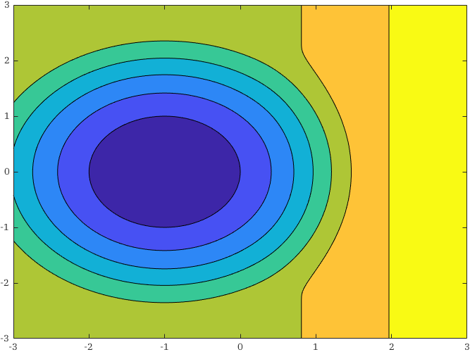
In Figure 2 we see the level sets (contours) of \(h\) and how both the unit circle centred at \((-1, 0)\) and the vertical line at \(x = 2\) are contours. So, we can define a new coordinate system where one of these coordinates is \(z = h(x,y)\) and, in these coordinates, the circle and vertical line are “flat.” That is, \[z = 0, \quad z = 2,\] correspond to the state being on the circle and vertical line respectively. We then can use simpler control design techniques to render these locally (un)stable.

The same cannot be easily done in the real-analytic case. It is tempting to integrate the differential \[((x + 1)^2 + y^2 - 1)\, dh_1 + (x - 2)\, dh_2,\] but the resulting analytic function is \(0\) on both sets. Unfortunately, the alternative, \[((x + 1)^2 + y^2 - 1)\, dh_1 - (x - 2)\, dh_2,\] is not locally closed and so cannot be integrated to produce a real-analytic function. There does, in fact, exist a real analytic function that satisfies the boundary conditions. Can you think of it?