How to Sample on Manifolds: Part 2
Consider the unit sphere \(\mathbb{S}^2 \subseteq \mathbb{R}^3\) and a (non-constant) random variable \(X: \mathbb{S}^2 \to \mathbb{R}.\) How can we sample points on \(\mathbb{S}^2\) according to this random variable with the surface area measure?
Let us attempt the approach described in Part 1 with a little more detail. Define the projection \(\pi: \mathbb{R}^3\setminus \{0\} \to \mathbb{S}^2\) by \[\pi(x) = \frac{x}{\| x \|}.\] Suppose that, without loss of generality, \(X \geq 0.\) Define the open set \[D = \left\{ x \in \mathbb{R}^3 \colon 0 < \| x \| < 3\sqrt[3]{X(\pi(x))}. \right\}.\]
Claim: The probability of a point being sampled in an open set \(U \subseteq \mathbb{S}^2\) according to random variable \(X\) is equal to the probability of a point being uniformly sampled in the open set \(\pi^{-1}(U) \subseteq D.\)
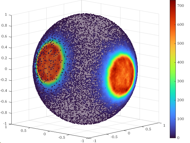
To show this is true, we must show that the volume of \(\pi^{-1}(U)\) is precisely equal to the probability we expect for points to be observed in \(U.\) The volume of \(\pi^{-1}(U)\) in spherical coordinates is \[\int_{\pi^{-1}(U)} r^2 \sin(\phi)\, dr \wedge d\theta \wedge d\phi.\] It suffices to consider rectangular open sets of the spherical coordinate system. Restricting our attention to sufficiently small sets where \(\theta \in (-\theta_0, \theta_0)\) and \(\phi \in (-\phi_0, \phi_0)\) vary independently, write \[\int_{\pi^{-1}(U)} r^2 \sin(\phi) \, dr \wedge d\theta \wedge d\phi = \int_{-\phi_0}^{\phi_0} \int_{-\theta_0}^{\theta_0} \int_{0}^{3\sqrt[3]{X((\theta, \phi))}} r^2 \sin(\phi)\, dr\, d\theta\, d\phi.\] Evaluate the inside integral, \[\int_{\pi^{-1}(U)} r^2 \sin(\phi)\, dr \wedge d\theta \wedge d\phi = \int_{-\phi_0}^{\phi_0} \int_{-\theta_0}^{\theta_0} \sin(\phi) X(\theta, \phi)\, d\theta\, d\phi.\] And observe that the right-hand side of the integral is in fact precisely \[\int_{\pi^{-1}(U)} r^2 \sin(\phi) dr \wedge d\theta \wedge d\phi = \int_{U} X(\theta, \phi) d\theta \wedge d\phi.\] Since this holds for any sufficiently small open set in the basis for the topology on \(\mathbb{S}^2,\) it will hold for any open set on \(\mathbb{S}^2.\) As a result, we expect uniformly sampling \(D\) and projecting down onto \(S^2\) through \(\pi\) will produce a family of points that are distributed according to \(X.\) Here are points distributed by the sum of two normal distributions on \(\mathbb{S}^2\) sampled using this method.
Unfortunately this method relies on the existence of a projection map \(\pi\) and a clever nonlinear transformation of \(X\) — here that was \(3 \sqrt[3]{X}\) — to correct for the nonlinearities introduced by the measure of volume in the preimage of \(\pi.\) Although it is in theory doable to generalize this approach to arbitrary manifolds (since all manifolds can be embedded in some real space), producing the nonlinear correction is tedious. In the next post, I will consider the more general case of an abstract manifold not embedded in \(\mathbb{R}^n.\)