Suppose we wanted to generate points on the unit circle whose weight is given by the random variable \(X: \mathbb{S}^1 \to \mathbb{R}.\) How would we go about this? If we are using the “angle” measure — recall measures compute “volumes” of subsets in a space — on \(\mathbb{S}^1,\) which is a multiple of the ambient measure in \(\mathbb{R}^2,\) then we consider the random variable \(Y: [0, 2\pi) \to \mathbb{R}\) given by \[Y(\theta) = X\left( (\cos \theta, \sin \theta) \right).\] It suffices to produce samples from the random variable \(Y\) defined now on a half-open interval of \(\mathbb{R}\) and map them forward onto \(\mathbb{S}^1.\)

Easy. This takes advantage of a nice property of \(\mathbb{S}^1\): there exists a measureable map from \([0, 2\pi)\) into \(\mathbb{S}^1\) where the angle measure on \(\mathbb{S}^1\) is equal up to a multiple of the pushforward of the Lebesgue measure on \([0, 2\pi).\) The way we measure length on \(\mathbb{S}^1\) matches up to a constant multiple the way we measure length on \([0, 2\pi)\) and map that to \(\mathbb{S}^1.\) This is not always so easy to do.

Consider the unit sphere \(\mathbb{S}^2 \subseteq \mathbb{R}^3\) constructed in \(\mathbb{R}^3\) in the standard way with random variable \(X: \mathbb{S}^2 \to \mathbb{R}\) that is constant. This is what one might think of as the uniform probability distribution as it assigns the same weight to all points. One approach to sampling is to consider the map \[\begin{aligned} \varphi: &[0, 2\pi) \times \left[\frac{-\pi}{2}, \frac{\pi}{2}\right] \to \mathbb{S}^3\\ &(\theta, \phi) \mapsto \left(\cos\theta \sin\phi, \sin\theta \sin\phi, \cos\phi\right). \end{aligned}\] What would sampling random numbers in \([0, 2\pi) \times [-\pi/2, \pi/2]\) according to the weight \(Y(\theta, \phi) := X(\varphi(\theta,\phi))\) product? Let us see what happens empirically. If we sample uniformly in \([0, 2\pi) \times [-\pi/2, \pi/2]\) and map through \(\varphi,\) this is what the sample points look like.

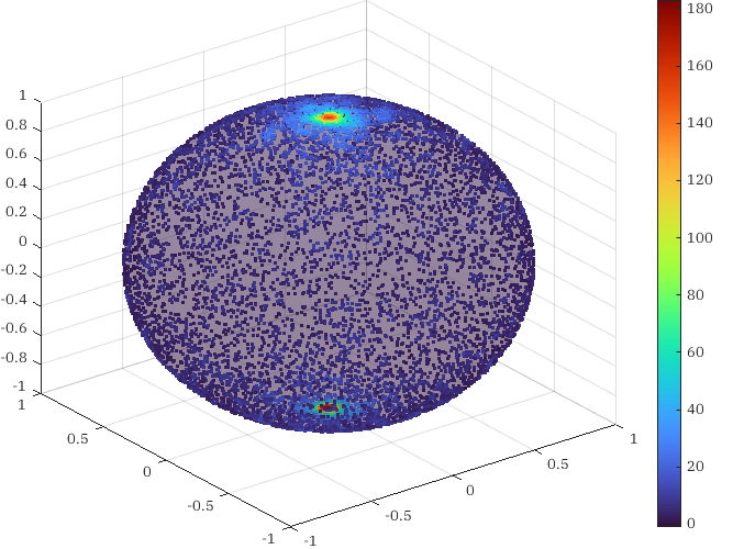
Note the clustering around the poles. This is not what we consider a uniform distribution on \(\mathbb{S}^2.\) Of course, that is because of our preconcieved notion of what “uniform” means!

The measure induced by \(\varphi\) is not the measure we are expecting on \(\mathbb{S}^2.\) The measure we expect on \(\mathbb{S}^2\) is the one that, for any open or closed set \(U \subseteq \mathbb{S}^2,\) computes the surface area of \(U\) when viewing \(\mathbb{S}^2 \subseteq \mathbb{R}^3\) as sitting in \(\mathbb{R}^3.\) We define this measure on \(\mathbb{R}^3\) using the volume form \(dx \wedge dy \wedge dz.\) For any open subset \(U \subseteq \mathbb{R}^3\) the integral \[\int_{U} dx \wedge dy \wedge dz,\] measures the volume of \(U.\) If we equip \(\mathbb{R}^3\) with a Riemannian manifold structure — the standard one — then we can induce a volume form on \(\mathbb{S}^2\): the form that, when integrated on a surface of \(\mathbb{S},\) measures the surface area. The volume form is explicitly given by (using the Euclidean metric here) \[\begin{aligned} dG &= \left( \frac{1}{\sqrt{3}} \partial_x + \frac{1}{\sqrt{3}} \partial_y + \frac{1}{\sqrt{3}} \partial_z \right) \,\lrcorner\, dx \wedge dy \wedge dz\\ &= \frac{1}{\sqrt{3}} \, dy \wedge dz - \frac{1}{\sqrt{3}} \, dx \wedge dz + \frac{1}{\sqrt{3}} \, dx \wedge dy. \end{aligned}\] Integrating this \(2\)-form over an open subset of \(\mathbb{S}^2\) computes the surface area of that set. How does this compare with the measure induced by \(\varphi\)? Well the problem is that it doesn’t induce a measure we expect. In fact, it doesn’t even induce a volume form on \(\mathbb{S}^2\)! The map \(\varphi\) isn’t invertible on all of \(\mathbb{S}^2.\) On the open set where it is invertible, the volume form of \(\mathbb{R}^2,\) \(d\theta \wedge d\phi,\) mapped into that open set looks like \[\begin{aligned} d\theta \wedge d\phi &= \left( \frac{1}{1 + \left(\frac{y}{x}\right)^2} \left( -\frac{y}{x^2} dx + \frac{1}{x} dy \right) \right) \wedge \left( \frac{1}{\sqrt{1 - z^2}} dz \right)\\ &= -\frac{y}{(1 - z^2)^{3/2}} dx \wedge dz + \frac{x}{(1 - z^2)^{3/2}} dy \wedge dz \end{aligned}\] Note the singularity at both poles where \(z \to \pm 1.\) This suggests that, for the same movement in the \(z\)-direction, the value of that length grows the more we approach the two poles.

So how do we sample on \(\mathbb{S}^2\)? One particularly straightforward strategy is the following. Randomly sample numbers uniformly distributed over the space of points \(x\in\mathbb{R}^3\) satisfying \[1 \leq \| x \| \leq 2.\] This is easy, since we can simply uniformly sample a cube \([-2, 2]^2\) and filter the points that satisfy the constraint. Normalize these points. The distribution of these normalized points, which now live on the sphere, will be uniform over the induced measure on \(\mathbb{S}^2.\) For visual evidence see,

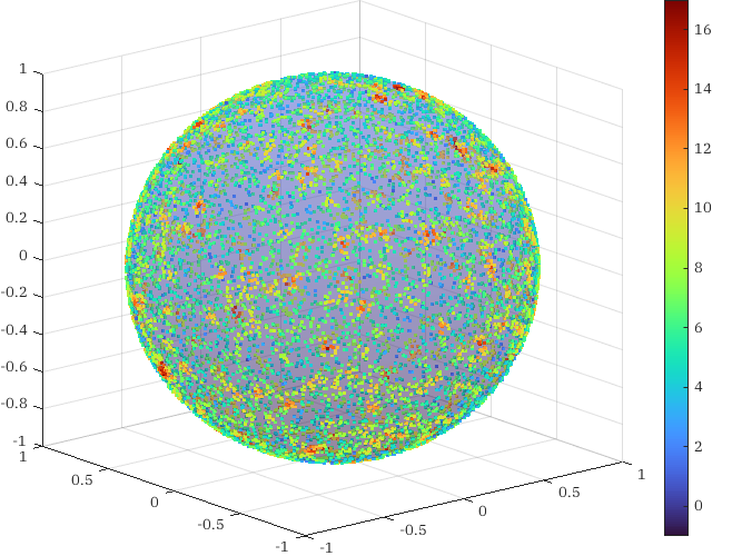
Why does this work? If we pick any two open subsets \(U_1,\) \(U_2 \subseteq \mathbb{S}^2\) that have the same area, as per the induced measure, the open sets \(V_1,\) \(V_2 \subseteq \mathbb{R}^3\) that are projected onto \(U_1\) and \(U_2\) by the normalization function \(\|\cdots\|\) also have the same volume in \(\mathbb{R}^3\) as per the standard measure. Uniformly distributed points over that volume are projected into uniformly distributed points over \(\mathbb{S}^2.\)

What if we have a random variable \(X: \mathbb{S}^2 \to \mathbb{R}\) where the weight is not constant, so we wish to sample a non-uniform distribution on \(\mathbb{S}^2.\) Can we generalize this approach? More on this in the next post.